PalmSearch Part 3: Model Inference and Counting Palms
TL; DR
This is a multi-part series on using single-shot ML algorithm to answer a very simple question: does Thousand Palms, CA live up to it’s name?
- Part 1: How hard could it be to grab some satellite data from Google Maps?
- Part 2: Big data meets bad data - generating a training dataset
- Part 3: Running YOLOv11 - How many palms are there in Thousand Palms? Did we even need to count?
In this post I will be revealing training a YOLO model on our training dataset and sharing the results. Spoiler alert - there are at least 1000 palms in Thousand Palms. It turns out that the palm tree density is roughly 1 per household.
Introduction:
I had originally considered trying to run YOLO on my AMD GPU, but the ease of working with NVIDIA and PyTorch won out. Due to my GTX 970 GPU only having 3.5 GB of VRAM, I was limited to using the YOLOv11-nano pre-trained model. The provided instructions from Ultralytics do a good job implicitly highlight how far applying deep learning algorithms have come and why Python is so popular for interfacing with deep learning models.
from ultralytics import YOLO

# Load a model
model = YOLO("yolo11n.pt")  # load an official model

# Predict with the model
results = model("<image-filename>")  # predict on an image
To pull the annotated dataset from Roboflow, I grabbed my API key and pulled the workspace/project information. As always, never share API keys in Git - I am using a .env file in my workspace and an exception in .gitignore to make sure it does not end up in the commit history.
 # add Roboflow api to .env file in main git repo
rf = Roboflow(api_key=ROBOFLOW_API_KEY)

workspace = rf.workspace("treesearch")
project = workspace.project("palms-nfvyz")
version = project.version(3)
dataset = version.download("yolov11")
The documentation from Ultralytics is very handy and outlines very clearly the various parameters that can be used when setting training parameters. Training the model was straightforward, starting with 200 epochs.
    # Load a pretrained YOLO model (recommended for training)
    model = YOLO("yolo11n.pt")  # only nano model fits in VRAM

    # Train the model using data from Roboflow and verify against validation set
    results = model.train(
        data=f"{dataset.location}/data.yaml",
        epochs=200,
        resume=False,
        name="palm_search",
    )
    results = model.val()
We can see that only after a few epochs, the pre-trained model is already reaching a reasonable 50-50:
Logging results to /home/david/git/yolo11/runs/detect/palms_search3
Starting training for 200 epochs...

      Epoch    GPU_mem   box_loss   cls_loss   dfl_loss  Instances       Size
      1/200      2.62G      2.562      4.389      2.248         22        640: 100%|██████████| 28/28 [00:10<00:00,  2.58it/s]
                 Class     Images  Instances      Box(P          R      mAP50  mAP50-95): 100%|██████████| 2/2 [00:00<00:00,  4.15it/s]
                   all         49        229    0.00127      0.118     0.0198    0.00421

      Epoch    GPU_mem   box_loss   cls_loss   dfl_loss  Instances       Size
      2/200      2.59G      2.227      3.548      1.888         10        640: 100%|██████████| 28/28 [00:10<00:00,  2.67it/s]
                 Class     Images  Instances      Box(P          R      mAP50  mAP50-95): 100%|██████████| 2/2 [00:00<00:00,  4.19it/s]
                   all         49        229    0.00324      0.191    0.00503    0.00127

      Epoch    GPU_mem   box_loss   cls_loss   dfl_loss  Instances       Size
      3/200      2.62G      2.232      3.403      1.867         19        640: 100%|██████████| 28/28 [00:10<00:00,  2.68it/s]
                 Class     Images  Instances      Box(P          R      mAP50  mAP50-95): 100%|██████████| 2/2 [00:00<00:00,  4.14it/s]
                   all         49        229      0.507     0.0417     0.0527    0.00973

    ...

      Epoch    GPU_mem   box_loss   cls_loss   dfl_loss  Instances       Size
     10/200      2.58G      1.973      2.395        1.8         47        640: 100%|██████████| 28/28 [00:10<00:00,  2.70it/s]
                 Class     Images  Instances      Box(P          R      mAP50  mAP50-95): 100%|██████████| 2/2 [00:00<00:00,  4.77it/s]
                   all         49        229       0.45      0.503      0.484      0.155
In my testing, I found that there was not much advantage going beyond 200 epochs due to the issues I identified in the previous post on the quality of the dataset labeling. Still, this is a good enough model to start playing around with to answer my original research question: “Are there at least 1000 palms in Thousand Palms, CA?”.
Interlude: Fermi Estimates and the power of thinking in orders of magnitude
Before I divulge the results, I wanted to take a brief pause and try to guess how many palms we would expect in the spirit of Enrico Fermi’s order of magnitude calculations. As a physicist, Fermi has always been a fascinating historical figure to read about due to how well-versed he was in both theoretical and experimental physics. A Fermi estimate is essentially an estimate that rounds quantities to the nearest order of magnitude. We can get an estimate for the number of palms in Thousand Palms by considering the demographics and our best guess for the number of palms per house. In 2022 Thousand Palms had ~8200 people, or 2700 households. Let’s call that $10^3$ households. Then we need to decide how many palms per household - some people have no palms, and some families may have 3+ palms per home. So the average is probably on the order of magnitude of 1, not 0.1 or 10 per household.
So purely based on a Fermi estimate, we would expect at least 1000 palms in Thousand Palms! That seems more reasonable than only 100 or 10,000. Now, onto the actual results to see if our estimate bears out.
Model Results:
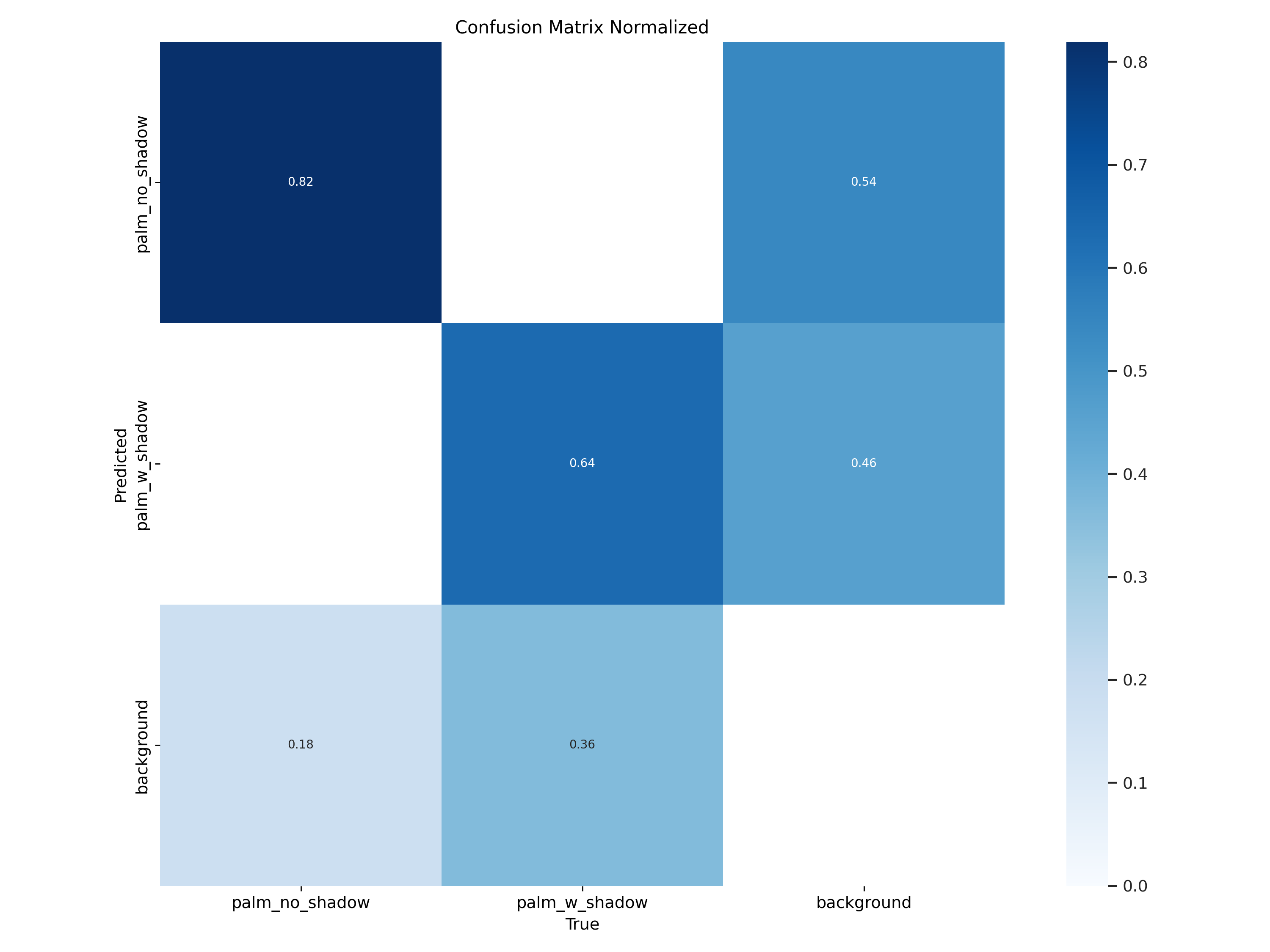
The results were more or less in line with my expectations: the model could reliably find both types of palms, but there were definitely many cases of missing palms. Not surprisingly, there was no cross-correlation between the two classes (likely due to the difference between symmetric/asymmetric bounding boxes used in the two classes), but there was substantial number of detections in the training dataset that the model missed.
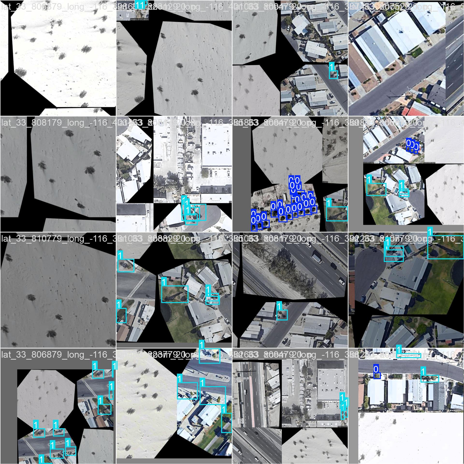
Looking at some of the model outputs on the training data, it is quite clear that palm trees without a significant amount of background noise or adjacent trees/shrubbery are easily detected, but the model struggles with complex shadows/structures. I was pleased to see that light/telephone poles with their distinct shadows are not immediately popping up as false positives. However, I raised many of these issues in Part 2 during classification on the training dataset that increasing the number of training images by 5-10x and splitting out the classifier classes for complex shapes or double/triple adjacent palms would likely improve the recall by standardizing the bounding box sizes within the class.
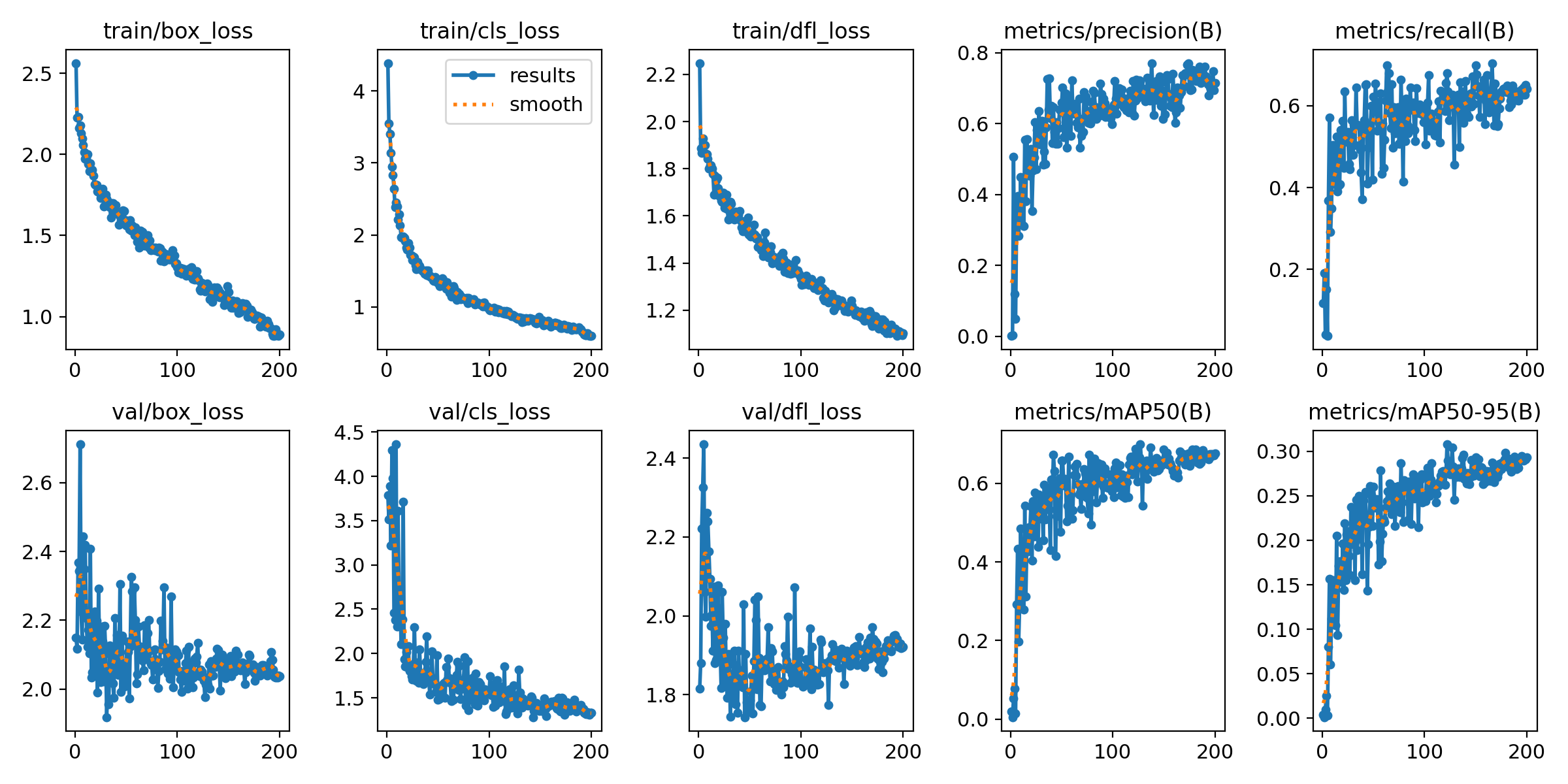
We can look at the model performance metrics to better quantify these qualitative observations - box loss, classification loss (cls_loss), distributed focal loss (dfl_loss), precision, recall and mAP. We can see that after 200 epochs the classification loss appears to saturate along with the precision/recall curves, the box loss and dfl_loss do not appear to be reaching saturation. This highlights that the model is not appropriately trained on the more difficult detection cases in the training set. This highlights my initial hunch that the ground-truth encoding in training dataset was insufficient to reach high precision ($P,R > 0.8$), and the model could benefit from a larger validation dataset to decrease the epoch-to-epoch variation.
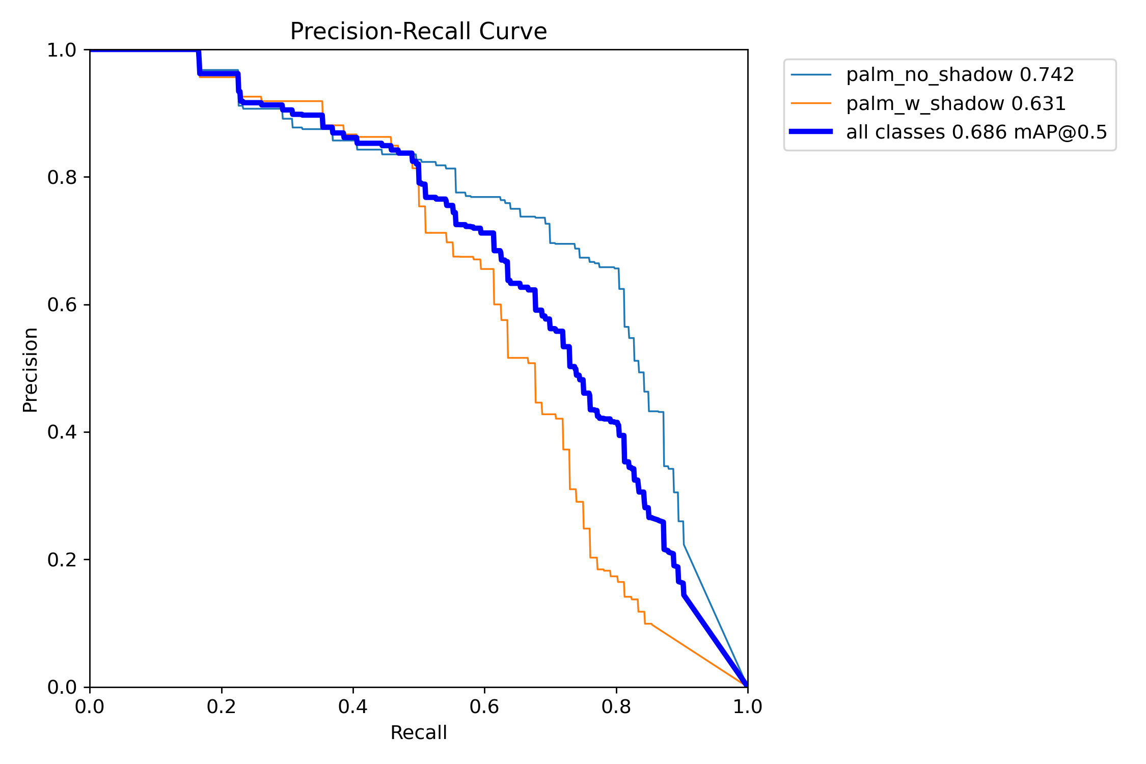
Based on the precision-recall (PR) curve, we can see that the model achieves a reasonable detection threshold, but would require significant improvements to the dataset to reach a production-level model. Again, it was the palm_no_shadow used to encode the larger date palms or fan palms with no good shadow to detect that significantly outperforms the other class. Both curves appear to diverge around $R=0.5$, suggesting that the palm_w_shadow class struggles to encode edge cases in the dataset.
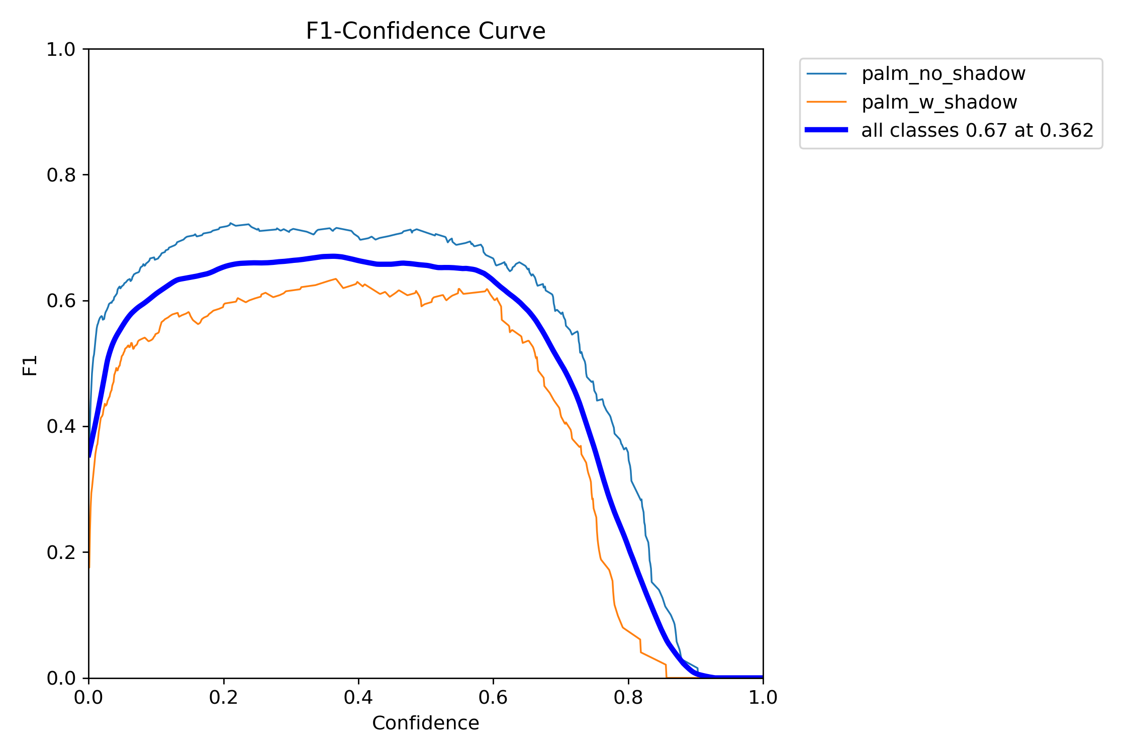
The F1 score (harmonic mean of P and R, $F1 = 2 PR/(P+R)$) highlights again that there are two regions of improvement of the model - extending the F1 plateau to higher confidence would require better control of the training bounding boxes used on both palm detection classes. Increasing the F1 score plateau value across the board would likely come with increasing the training and validation dataset size and improving the quality the of the ground-truth bounding boxes used. However, sicne I am using this model as a toy-project and not a production tool, the model performance is likely sufficient and I will be considering detections at the confidence $>0.25$ level.
Putting the model to work: Inference and Palm Tree Counting!
Finally, we can get to inference on the pre-downloaded grid of images from the Google Maps API around Thousand Palms from Part 1. I set up a simple loop through a new dataset on Thousand Palms, CA that I generated in Part 1, and ran inference on each image in the grid. I saved any images with a detection and also appended the results to a pandas dataframe for further analysis downstream. In particualar, I embedded the lat/long pairs in the filenames, so saving the images was helpful in extracting where exactly each of these detections occur.
First, since the grid generated did not exactly follow what Google Maps claimed the town boundary of Thousand Palms to be, I had to first screen to make sure that the lat/long coordinates of the grid tile fit within the town limits. The Google Maps API geocoding allows for city/town level lookups and will return a pair of coordinates for the bounds. Limiting the bounds to a pair of lat/long coordinates means that only trapezoid shapes are allowed, which is sufficient for this level of work. Inference was much faster than training, averaging around 8 ms per image.
During the loop through all of the grid images that matched our geocoded lat/long grid, I ran inference on each image and only kept images where there was a detection. Converting the output to a Pandas dataframe made it easy to analyze later as all of the important paramters were stored (location, bounding box size, confidence, etc.), to which I also added the filename so that I could parse the lat/long pairs.
Based on the grid of images I pulled, I found that there may be up to 3366 palms in Thousand Palms using the default confidence level of 0.25. This is in the ballpark for what I expected based on the number of households using a Fermi estimate. Unsurprisingly, the distribution of the inference confidence levels largely match the shape of the F1-score from training.
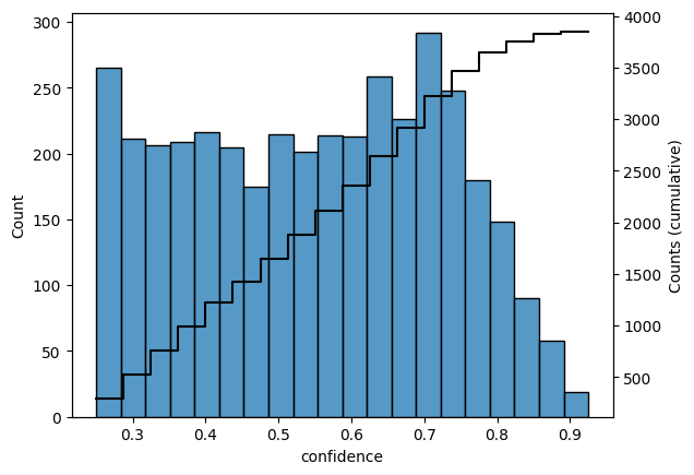
The 3366 number comes from all detections down to the lowest confidence level used. I’ve made a quick summary table here of the results at different confidence levels.
| Confidence Level | Palm Tree Count |
|---|---|
| 0.25 | 3366 |
| 0.3 | 3047 |
| 0.4 | 2506 |
| 0.5 | 1972 |
| 0.6 | 1442 |
| 0.8 | 208 |
Obviously there is some wiggle room here, but I think it is safe to say that even at a high confidence threshold of 0.6, there are still at least a thousand palm trees in Thousand Palms, CA. Being generous, at the lowest confidence level, the average palm tree density per household is $\sim 1$.
Next steps and Lessons Learned?
Thank you for reading this far. Although none of the individual steps in this project were that complex, it took about a week of finding an odd hour or two here and there to get it done (and almost more time to write it up). I am fascinated by how far open-source object detection and segmentation models have come in the last five years, but like any ML application the reliance on a large, clean dataset generation still remains a major challenge. Roboflow’s interface for labeling, including the ability to use a single-shot model to kickstart detection was neat and I could see how the paid tier would be useful for developing models for internal tooling or production.
If you are curious, I have not yet decided what next steps if any I want to take this project beyond the simple proof of concept. I spent $27.41 on API calls, so there is still plenty of GCP credit to spend on other cities/towns. Some ideas are listed below:
- Compare other “palm” flavored cities in SoCal to get a palm-per-capita/palm-per-household metric
- Play around with geospatial encoding to generate annotate palm tree map.
- Try this same exercise with Google Street View imagery instead for higher fidelity detection
- Try training a RCNN two-shot model on the dataset to compare performance
- Commercialize this and sell the data to all of the tree trimming companies that keep dropping flyers by my house