PalmSearch Part 2: Building up a Training Dataset of Palm Trees
TL; DR
This is a multi-part series on using single-shot ML algorithm to answer a very simple question: does Thousand Palms, CA live up to it’s name?
- Part 1: How hard could it be to grab some satellite data from Google Maps?
- Part 2: Big data meets bad data - generating a training dataset
- Part 3: Running YOLOv11 - How many palms are there in Thousand Palms? Did we even need to count?
In this post I will be explaining the steps used to annotate a training dataset for palm tree detection in Google Maps satellite imagery, along with the pitfalls and lessons learned.
Introduction:
A quick look on Google Maps showed that while Thousand Palms, CA is a fairly small community in the greater Coachella valley region, there are plenty of other communities nearby with a high degree of palm trees. I pulled the coordinates for a densely populated region of Palm Springs to get a good mix of residential, commercial and recreation areas (parks, golf courses, etc.) for training. I used a 50x50 grid for this to get enough images for a training dataset.
Due to time constraints, I went into the annotation portion of the project only looking to map $\sim$100-200 images for training to see how well initial training would go with a YOLOv11 model. For training, I used the Roboflow free tier and created a public project.
Uploading images was fairly straightforward using the web interface or the CLI. Adding files with the CLI was as simple as adding roboflow to the current Python environment using pip install roboflow, and then following the Roboflow instructions roboflow import -w <workspace-name> -p <project-name> <path/to/data/>. I found grouping different satellite image grids into subfolders was easier to manage with the import process as if I wanted to add more images in the future I could track where each image came from if I was worried about oversampling a given region.
Annotating the Palm Trees
Going in, I had decided that I wanted to be using YOLOv11 for training and inference. The first challenge was determining how granular to be with the annotations - in Southern California I’ve noticed that the dominant and most prominent palm trees tend to be Mexican/California fan palms (typically can grow very tall and skinny), or date palms (with their long leaves and broader canopies). There are also other less common palms - royal palms or King/Queen palms that we could separate out into separate classes.
Flipping through a bunch of images manually to see what I was dealing with, I found that there were three main issues to work around that came over the course of annotating:
- How many palm tree classes to use? Separate date/fan palms or use the same class?
- How to handle orientation with a rectangular bounding box? What about palms and shadows oriented at 45 degrees?
- How should we handle multiple adjacent palms?
Setting up Palm Tree Classes
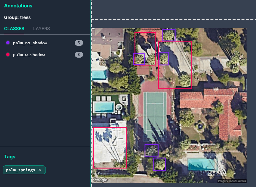
The first problem was dealing with how many classes to setup. Each additional class would require at least a few hundred instances to train on. From poking through and drawing the bounding boxes, it appeared that I could split the classifications into two types: tall palms with a clear shadow (palm_w_shadow), and large palms that may or may not had a clear shadow (palm_no_shadow). This essentially parallels the split between tall and skinny fan palms and the shorter but broader date palms, but also allows to us to add the other more rare palms into one of these two classifications.
It also helped that if a palm had an unclear or obscured shadow due to buildings or other trees, we could still categorize it as a palm_no_shadow. An example training image is shown below with the two different classes:
Palm Tree Orientation
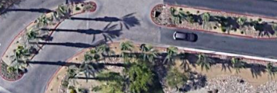
The next problem that kept coming up as I went through the grid of training images was shadow orientation. Google Maps does not have the ability that Google Earth does to look at satellite images taken at different times, so we are stuck using what Google serves as the “best” image available. If we luck out, the shadows are oriented along our pixel grid, making our bounding boxes nice and horizontal/vertically oriented. However, there is a significant chunk of the dataset that has shadows oriented at 45 degrees relative to our pixel grid; this is literally the worst case scenario because it makes our bounding boxes large and introduces significant overlap when we have palm trees spaced close together.
By the time I reached the point where I had seen enough of these palm tree shadows oriented at 45 degrees, I had already labeled enough into the palm_w_shadow class that I felt like it was going to be too much work to go back and revise. In retrospect, the ideal solution would be separate out the 45 degree palms into their own class so our original palm_w_shadow class would just consist of palms with nice horizontal/vertical bounding boxes that are nice and tight around the subject material.
For the purpose of this project, the choice was not a deal breaker since I wanted to go for higher precision rather than high recall to get a lower bound on the number of palms in a given image grid. As I will get into more detail later, this ends up showing up clearly in the confusion matrix as the model tends to get confused with these large bounding boxes required to encapsulate the tree and its shadow.
Dealing with Multiple Palms:
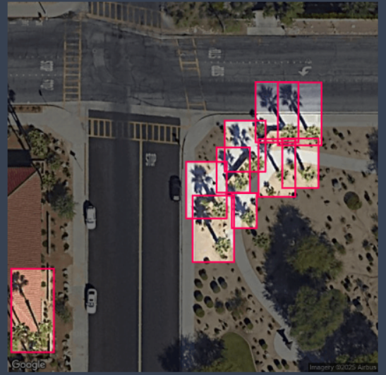
I found that I could not avoid multiple palms. Stylistically, it is quite common to see clusters of palm trees which give a nice aesthetic. However, for categorization this was quite a pain due to the difficulty of drawing tight enough bounding boxes to separate out the individual palms.
I decided to group 2-3 palms if I could not distinguish their bases even if their shadows were fairly distinct. Again, not ideal, but my logic behind it was that for the purposes of this project it’d be better to classify multiple palms as a single detection instead of avoiding it. Similar to above, this would probably be better split out into a new class for multiple_palms; however, similar decisions will need to be made as raised above if there are 2+ clustered palms with shadows that are oriented at 45 degrees to the pixel grid.
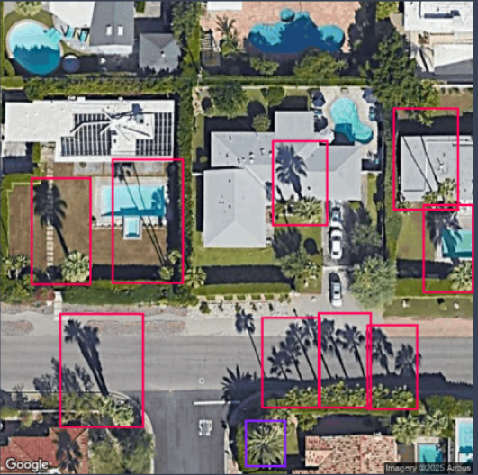
The other problem was that if the palms were too close to feel confident that the bounding boxes were unique enough, I just used the palm_no_shadow class on the canopy if the palm tree was large enough. This will show up for adjacent date palms in the next segment once we get around to training.
Summary:
I spent a few hours mucking around with looking at the data and then working on my two class annotations while putting on Parks and Rec in the background on a different screen.

As raised in the above sections, there were difficulties handling shadows oriented at 45 degrees to the pixel grid and multiple adjacent palms that couldn’t be nicely split into their own bounding boxes. They all ended up getting swept into the palm_w_shadow class, but if I were to redo it, I would split them out. This would have the benefit that during training we would have the granularity to identify if there was significant confusion between classes. On the flip side, avoiding overfitting would require at least 50-100 instances which would take a bunch more time to classify.
Lessons learned: ideally, we would have shadows aligned with our pixel grid for easy classification. Otherwise we should have split out the palms with shadows at a 45 degree angle to our pixel grid into a new class or done some kind of image rotation scheme at 45 degrees to get the shadows to align nicely with the bounding boxes. The second method would also have required some way to map the original image to a rotated version and preserve the pixel original pixel locations in case we wanted to grab the coordinates/location of the detected palm down the road.
Of course, this could all be avoided in a product type project where we could spend the money on nice satellite data where we could standardize the sun angle across the training and inference images… but spend more money is always a cop out answer.
The next step would be grabbing the dataset for local training on my old GTX 970 and learning the lessons above with dealing with edge cases in the classes.