Time Series Analysis: Fourier Transforms and Autoregression Approaches
TL;DR
I am a condensed matter physicist by training working with time-domain and frequency-domain spectroscopy, so I am biased towards thinking about just Fourier transforming everything. Time series analysis is an important and practical problem for data scientists and a number of excellent tools exist for analyzing and forecasting time series data. I break down my background with the Fourier transform and highlight statistical autoregression modeling to identify key components of time series and generate predictions.
At its core, time series data is broken up into slow and fast oscillatory components. The slow component represents the long-period background trend, typically with some seasonality or oscillatory component added on top. Combining these two aspects can be difficult from a mathematical modeling perspective and has real life impacts when trying to tune forecasts to realistic predict expected future data. For the complex systems around us - utilities, food and agriculture, commodities, fisheries - they are all impacted by the quality of our ability to forecast future expectations based on past data.
In this post, I highlight some of the mathematics behind why the Fourier transform is so great in physics and jump into both statistical approaches to time series analysis. I will get into other Bayesian models or machine learning based approaches in another post.
Back to school: Why Fourier Transforms are useful to understand quasiparticle lifetimes:
In condensed matter physics, we use Fourier transforms (FTs) extensively. Using various spectropscopic techniques (my expertise is in optical spectroscopy) to study the energy dependence response (remember that energy $E=\hbar \omega$) of a material and understanding the various features is a key component of doing good science.
If have some spectroscopic peak in frequency space ($\omega$) or equivalently energy space ($\hbar \omega$), the width of the peak will give the lifetime - a wider peak corresponds a short lifetime and vice versa. This can be measured via multiple spectroscopic probes - optics, scanning tunnelling spectroscopy (STS) or Angle resolved photoemission (ARPES). This is the basic framework that must be used to describe exotic phenomena like low-energy analogues of exotic particles (quasiparticles, Majoranas, plasmons, Higgs modes, etc. ). We can understand this by thinking of a quasiparticle existing as a Gaussian wave packet in the time domain - essentially a Gaussian/normal distribution with oscillatory components. A wave packet exists in between two limits: a infinitely short delta function or an infinitely long oscillatory term. The duality of the Fourier transform is that the more well defined the function is in time, the less well defined it is in frequency (or vice versa) means that the lifetime for the time-domain delta function is essentially 0, and the lifetime for the infinitely long lived oscillatory term at $\omega$ would be $\infty$.
In physics, we utilize the damped harmonic oscillator model frequently due to its ability to describe natural phenomena and deep mathematical understanding. For low energy physics (as opposed to particle physics), understanding the various energy scales and interactions of the electrons, lattice modes/phonons and energy transitions is key for establishing a baseline understanding of material properties and paves the way to do interesting applied physics/engineering applications.
I will get into the details in the next few sections, but the key point I want to make is that the Fourier transform and thinking in terms of a sum of harmonic component is extremely powerful for understanding time domain/time series data. At the core, most of the models I will explore in this post are building upon the idea of the Fourier transform; however, if we are just interested in the amplitude and frequency of the harmonic components of our signal, we can do away with much of the complexity and “finickiness” of the full Fourier transform with simpler approaches while still maintaining the key features of its predictive properties.
Fourier Transforming Time-Series Data:
I won’t go into too much detail about the Fourier transform (FT), but essentially decomposes a time domain input $x(t)$ in terms of a sum of sine/cosines.
$$ f(\omega) = \int f(t) e^{-i \omega t} dt $$
Generally, the FT is complex valued and can be represented as a magnitude and phase. For most time series applications, the phase information is generally not of primary interest unless there is interest in comparing the correlation of multiple harmonic terms present in the data.
Like the other transforms, FTs are extremely useful for decomposing noisy or complicated time domain signals to identify key harmonics or patterns. For example - take the NOAA Mauna Loa CO2 and CH4 data taken at daily and monthly intervals respectively.
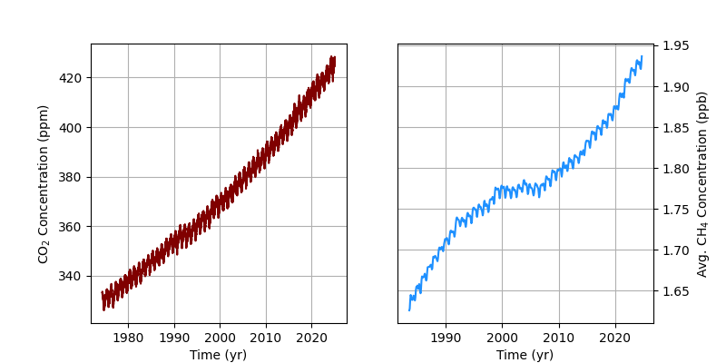
CO2 levels have known yearly seasonality due to the summer/winter seasonal pattern in the Northern hemisphere. However, making FTs useful in analysis requires knowing a few details of how to prepare the data before taking the FT. The main issue with taking a FT without a priori knowledge of the key harmonic components of the data (if there are any) is spectral leakage and handling large “DC” type terms (as opposed to the harmonic AC terms).
Spectral leakage commonly occurs in real life because sampling time series data always occurs over a finite window. The FT of a simple $\cos(\omega t)$ function in the time domain is a delta function $\delta(\omega)$, but for a finite sample window approximated by a rectangular window between $t=0$ and $t=t’$, our measured signal $S(t) = w(t) * x(t)$, is a convolution of our window function and the $x(t)$ original time domain signal. The convolution operator in the time domain $ w(t) * x(t)$ is equivalent to multiplication the frequency domain $w(\omega) x(\omega)$. The FT of a rectangle window with a width $\tau$ is a sinc function $\textrm{sinc}(\omega \tau/2)$1:
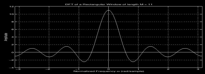
This means that even a single component harmonic signal $\cos(\omega t)$ will have distortion in the frequency domain if the sampling window does not include an integer multiple of periods.
Coupled with the spectral leakage issue that large DC components ($\omega = 0$) can have spectral leakage that obscures present harmonic terms. The simplest approach would be to subtract the mean from the time series data to remove the DC offset. We can work around this by assuming that the background is slowly varying signal of a polynomial form and subtracting off this background if a simple average over the sampled time window is insufficient to isolate all of the harmonic terms.
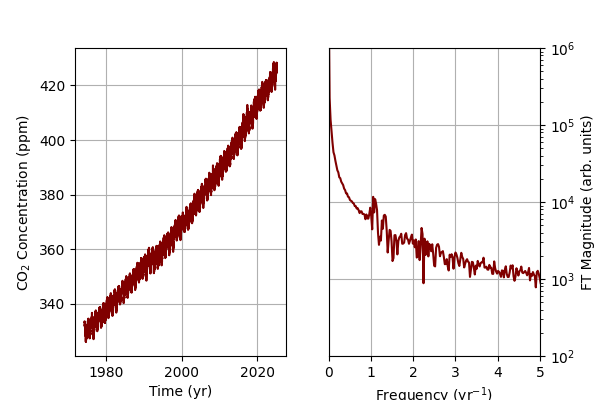
It is clear that the maroon CO2 data shows a clear seasonal trend, but there is also a huge exponential term underlying the data. If I take a naive FT, the spectral leakage of the DC background ends up largely obscuring the harmonic seasonal contribution we would expect around the $1 \, yr^{-1}$ mark.
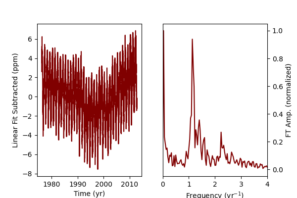
However, if we assume that there is a large DC background that we can model as a linear fit or a polynomial, we can subtract that off and consider just the harmonic terms. For the CO2 data, I just a linear fit, so the DC background is not perfectly removed. However, now we can see clearly that there is a clear seasonal trend in the FT that was not visible previously due to the spectral leakage of the DC background.
If I treat the CH4 data with a high order polynomial background subtraction ($n=4,5$), we can see that the background contribution at low frequency is almost completely removed.
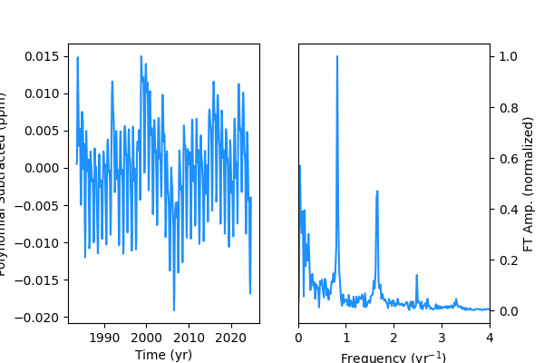
Interestingly, while in the CO2 data we have a clear component at 1 $yr^{-1}$, the methane data shows a principle harmonic slightly at 0.8 $yr^{-1}$. This may be due to the differences in CO2 seasonal variation driven by plant biomass uptake in the northern/southern hemispheres vs. absorption and the mean lifetime of methane.
However, while Fourier analyis is excellent for identifying key harmonic terms in time series data, making predictions and forecasting is not as straightforward. In particualr, when dealing with time series data that can be generalized to a background term, one or more well defined harmonic terms, and noise, a full Fourier analysis tends to be more complex than is necessary. The details of spectral leakage, windowing, background subtraction, etc. get to be more complicated when trying to dive into more than just simple key harmonic analysis. I would recommend readers look at Fourier Analysis of Time Series by Peter Bloomfield for more details.
Auto-Regression and Moving Averages:
One of more common ways to handle time series data is to combine auto regression and moving averages to understand data that shows both a random noise component and some underlying trend. A common statistical model used for time series analysis is the ARIMA model, which stands for “autoregressive integrated moving average” commonly found in statistics and economics.
ARIMA Theory
Autoregression refers to the correlation of a data point $i$ with previous points, denoted by the order $p$: $$ X_i = \Sigma_{n=1}^{p} a_n X_{i-n} + \epsilon $$ where $a_n$ are the correlation parameters, $X_i$ are the observed data points and $\epsilon$ is a random white noise term. The autoregression models are referred to by the order, i.e. AR(0) for a model with no correlation between terms, such as a noise only model, and AR(1) for the first order model which only considers the previous data point, etc. Autoregression does assume that the time series data is stationary, in that the mean/variance do not change with time. I’ll explore the more general ARIMA model below. The main weakness of autoregression is that it does not handle spikes or impulsive features well, but forms the foundation of many unsupervised machine learning models (NLP, LLM).
The moving average (MA) component of ARIMA acts like a low-pass filter, averaging some $N$ points on a sliding scale. The MA behaves like a convolution of the time series data and a rectangular window in time, which is multiplication in Fourier space. Depending on the sampling rate, time series data can be particularly noisy - using MA to handle trends is a powerful tool and can help separate out the background signals.
The “I” integrated term in ARIMA is the magic component that transforms the data to removing the background trend via differencing point to point (or some $n$ points, depending on the order) to generate a modified stationary time-series. The idea behind differencing is that assuming that the time series sampling rate is much faster than the background trend rate of change, the background can be approximated as a constant between two adjacent time series points. Common types of non-stationarity in time series come from a trend in the mean or shocks in a system that does not demonstrate mean-reversion.
Applying ARIMA to the Mauna Loa CO2 data
Let’s start by using a simple ARIMA approach to the Mauna Loa CO2 data. ARIMA models are referred to by the parameters $(p,d,q)$: $p$ is the AR order as the number of time lags, $d$ is the degree of differencing, and $q$ is the order of the moving average. So ARIMA(1,0,0) would be equivalent to the AR(1) model referred to above.
We can start by looking the autocorrelation function (ACF) and partial autocorrelation function (PACF) of our CO2 dataset.
import statsmodels.api as sm
import pandas as pd
import numpy as np

# load the co2 data from the repository
co2 = pd.read_csv(
    "data/co2_daily_mlo.csv",
    skiprows=32,
    names=["year", "month", "day", "timestamp", "ppm"],
)
data = co2["ppm"].astype(float)

fig = plt.figure(figsize=(8, 10))
ax1 = fig.add_subplot(211)
fig = sm.graphics.tsa.plot_acf(data, lags=40, ax=ax1)

ax2 = fig.add_subplot(212)
fig = sm.graphics.tsa.plot_pacf(data, lags=40, ax=ax2)
If we start with the data as is, we find that run into the same issue with the FT example above - the non-stationarity of the data completely renders the autoregression useless since the features of the underlying trend are obscuring the “true” autoregression. In the figure below, the top corresponds to the autocorrelation (ACF) and the partial autocorrelation (PACF) on 40 timesteps without any data treatment. As autoregression is only meant to model stationary data, the polynomial/exponential background in our CO2 data throws off the the autocorrelation calculation (i.e. it shows that all of the data points are highly correlated). To verify if the data is stationary, the Augmented Dickey-Fuller test (ADF) can be used to identify whether a unit root is present in the time series. However, if we do a first order difference (i.e. just diff our data array one time), the autocorrelation and partial autocorrelation plots clear up very nicely.
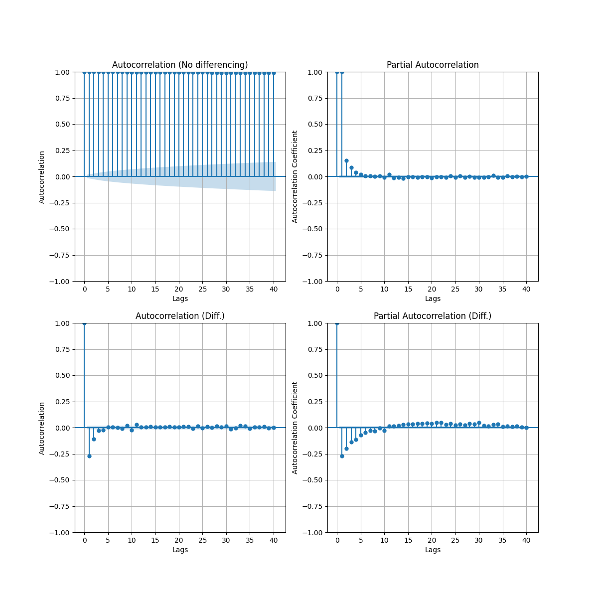
The ACF measures the correlation between points of time series - generally both the ACF and PACF are plotted with a lag of 0 which is always 1.0 since a data point is fully correlated with itself. The ACF plot can show whether the point to point noise in the time series data is random and if there is some moving average window that would be suit the data. The PACF considers the correlation explained by each additional lagged term.
Starting with ARIMA(1,1,1), we get the following output
res = sm.tsa.arima.ARIMA(data[0 : len(data)], order=(1, 1, 1)).fit()
print(res.summary())


                               SARIMAX Results
==============================================================================
Dep. Variable:                      y   No. Observations:                15552
Model:                 ARIMA(1, 1, 1)   Log Likelihood              -12825.460
Date:                Sat, 15 Feb 2025   AIC                          25656.920
Time:                        23:14:20   BIC                          25679.876
Sample:                             0   HQIC                         25664.523
                              - 15552
Covariance Type:                  opg
==============================================================================
                 coef    std err          z      P>|z|      [0.025      0.975]
------------------------------------------------------------------------------
ar.L1          0.3272      0.012     26.905      0.000       0.303       0.351
ma.L1         -0.7153      0.010    -74.833      0.000      -0.734      -0.697
sigma2         0.3047      0.002    161.709      0.000       0.301       0.308
===================================================================================
Ljung-Box (L1) (Q):                   0.66   Jarque-Bera (JB):             15382.40
Prob(Q):                              0.42   Prob(JB):                         0.00
Heteroskedasticity (H):               1.55   Skew:                             0.19
Prob(H) (two-sided):                  0.00   Kurtosis:                         7.86
===================================================================================
However, if we ask our model to generate predictions, we end up with a very flat response - the ARIMA model is unsuited to fitting the seasonal variation observed within the dataset.
Using Seasonal ARIMA (SARIMA):
This is where SARIMA comes in - ARIMA with an extra seasonal term. Note here that the seasonal component does not need to be of a single frequency. We can decompose our data first and determine the underyling trend with the seasonal component.
df = co2

# create new date-string to feed into Pandas datetime index
df["date_str"] = (
    df["year"].astype(str) + "-" + df["month"].astype(str) + "-" + df["day"].astype(str)
)
df["date"] = pd.to_datetime(df["date_str"])  # Handles various date formats
df = df.set_index("date")

data = df[["ppm"]]
print(data.head)

result = seasonal_decompose(data[:5000], model="additive", period=365)
fig = result.plot()
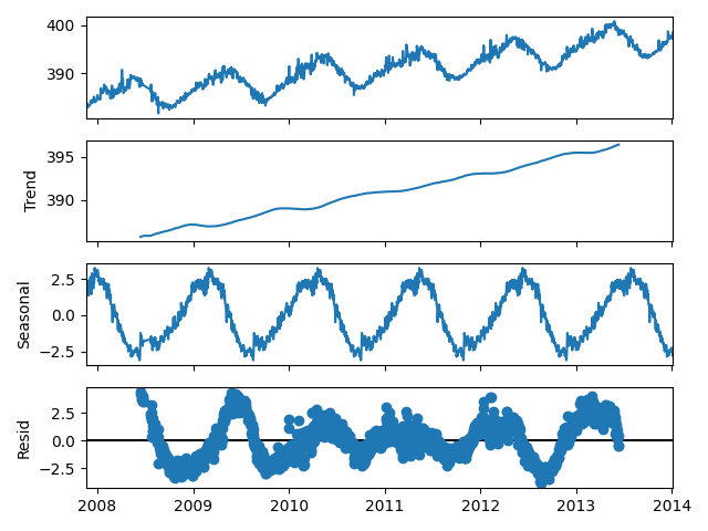
Using statsmodels built-in seasonal decomposition tool, we can easily separate out the long-term trend from the seasonal component. Here we see that the seasonal component is not a pure sine wave, so in the Fourier analysis there would be additional higher harmonic terms than just the base frequency at the $1 \, yr^{-1}$ fundamental frequency. Interestingly too - we can clearly see based on the magnitude of the seasonal and residual terms that we have found the northern and southern hemisphere seasonal split. The two curves are half a year out of phase with one another (seen by matching up peaks and troughs).
Setting up a simple SARIMA(1,1,1) model with the same (1,1,1) order for the seasonal component with the 365 day period, we can fit the data to generate some predictions. I was very happy to note when testing that the SARIMA function from statsmodels supports multithreading out of the box. However, out of the box, SARIMA only supports a single seasonal term, so if we want a better fit to our model to improve our predictions of the background trend and the seasonal effects, we will need to consider other models. If we had considered the phase effects of the Fourier transform with a sliding window, we would have likely observed that there were two out of phase components.
Conclusion
Hopefully I have convinced you that the Fourier transform is still very much relevant for any analysis of time domain data. For time series analysis, ARIMA and SARIMA are an excellent first tool to consider. However, complex harmonics or multiple seasonal terms are difficult to generate predictions for with these more basic models. In a later post, I would like to explore other statistical approaches or use machine learning based forecasting to handle the added complexity of real life data.